
Hello again.
Today I want to explain difference in averaging and low pass FIR filter. And actually I want to do it in some different way than it’s usually described in books.
Filter theory (and all digital signal processing theory) is quite complicated topic and there’s a lot of literature (on the internet or the books) that covers it. Here I just want to explain in few simple simulations (in time domain) the difference between averaging and low pass filter.
Well, to be honest averaging is also low pass filter. It’s actually a low pass FIR filter.
Why? First let’s take a look at digital FIR filter and see how it works.
Output of FIR filter is calculated with equation:
\(y[n] = b_0\cdot x[n]\;+\;b_1\cdot x[n-1]\;+\; …\;+\;b_N\cdot x[n – N]\)
b0, b1 … bN – coeficients of the filter
n – current sample number
x[n] – current input value (current sample value)
x[n-1], x[n-2], x[n-3] – previous sample values
y[n] – current output value of filter
The filter works in the loop, so when new sample arrives, we need to again calculate above equation with n increased by 1. So new sample will be multiplied by b0, previous sample (which last time was multiplied by b0) this time will be multiplied by b1, and so on. Just to make it clear I wrote down example with 4 coefficient filter, and to make calculations easier lets start at sample 10 (assuming that 9 previous samples were collected before).
The tenth output value of FIR filter will be:
\(y[10] = b_0\cdot x[10]\;+\;b_1\cdot x[9]\;+\;b_2\cdot x[8]\;+\;b_3\cdot x[7]\)
After collecting next sample (x[11]) the output of filter will be:
\(y[11] = b_0\cdot x[11]\;+\;b_1\cdot x[10]\;+\;b_2\cdot x[9]\;+\;b_3\cdot x[8]\)
After next sample (x[12]):
\(y[12] = b_0\cdot x[12]\;+\;b_1\cdot x[11]\;+\;b_2\cdot x[10]\;+\;b_3\cdot x[9]\)
Main problem in designing filter is selecting proper values for coefficients b0, b1 … bN. Those coefficients are responsible for filter characteristic shape. Choosing some values for those coefficients we can get low pass filter, choosing some other values we can get high pass filter, or low pass filter with different cut-off frequency etc. There’s a lot of methods for calculating those coefficients to get expected characteristic. We won’t talk about those methods in this article. For now, we just need to know that those values are responsible for filter characteristic.
Now let’s get back to averaging. We can calculate average value from N+1 consecutive samples using equation
\(y[n] = \frac{x[n]\;+\;x[n-1]\;+\;…\;+\;x[n-N]}{N+1}\)
There’s N+1 samples not N, because we are starting with x[n-0] sample (we can rewrite this equation for N samples, but with N+1 it will look nicer in next steps).
This equation can be written as:
\(y[n] = \frac{1}{N+1}\cdot x[n]\;+\;\frac{1}{N+1}\cdot x[n-1]\;+\;…\;+\frac{1}{N+1}\cdot x[n-N]\)
Now we can see that this equation is the FIR filter equation, with filter coefficients (b0, b1 … bN) values:
\(b_0=b_1=…=b_N=\frac{1}{N+1}\)
To show how average filter works I made some simulations. Those simulations were made in Python 2.7.13. If you want to play with those simulations on your own, contact me on e-mail or put comment below this article.
Let’s say that we have system that should measure some constant (or actually very low frequency) signal. We expect that on signal input we can also have some AC noise that we want to filter out.
Parameters of our system are:
- sampling frequency: 10000 Hz
- averaging filter length: 100 samples, which equals 10 ms
Averaging filter length is number of samples which are taken to calculate average value.
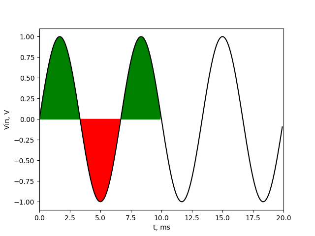
It’s easy to guess that if we put DC component to our averaging filter, the output of our signal will be just that DC value. More interesting thing is what happen when we put AC signal through our filter. In next picture i showed the signal of 1 V amplitude 100 Hz signal. The first 100 samples (first 10 ms) is taken to count the average value. I marked with green colour the values that are above 0, and with red the values that are below 0 in our averaging range.
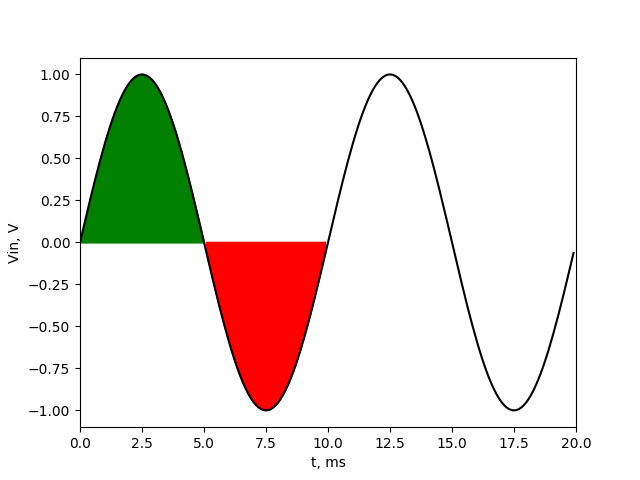 As we can see the average value of our 100 Hz noise signal in averaging range will be 0. The values above and below zero will compensate with each other. It doesn’t matter on which sample we’ll start our averaging. Below picture shows the same signal with averaging started in 10th sample (1 ms).
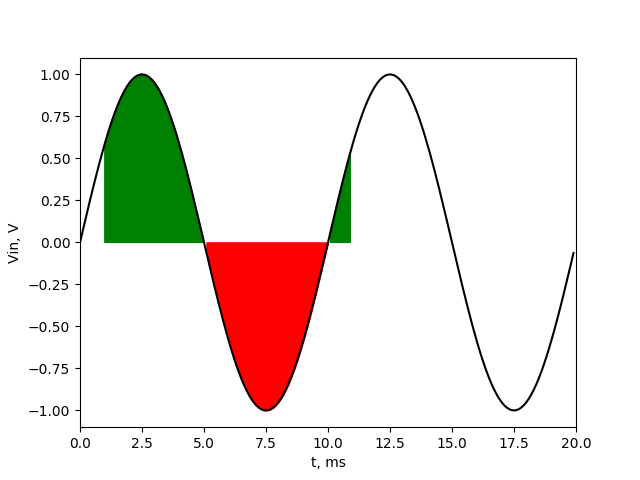
The sum of green field on the left and green field on the right is equal to red field, so after averaging that values, again we get 0 V. That’s why our filter will totally cut off that frequency.
Now let’s check what happen if we put 200 Hz signal into our filter. 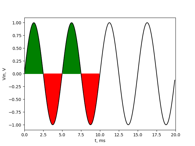
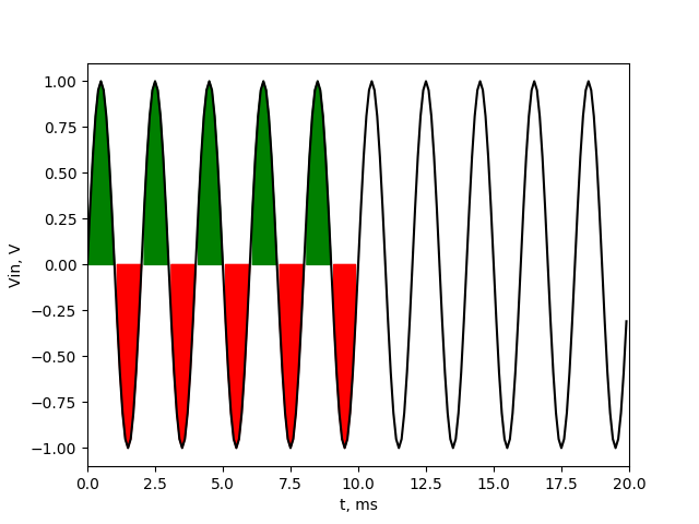
And again we can see that after averaging we’ll get just DC component of our signal. This will works for all signals that are integer multipliers of 100 Hz (all of those frequencies will be totally cut off). 100 Hz is frequency which period is exactly equal to averaging filter length. Below picture shows the the signal of 500 Hz and again the green values are equal to red values, so after averaging we’ll get 0 V at output.
But what’s happen when we have noise frequency that is not integer multiplier of 100 Hz, like 150 Hz?
Now we can see that the sum of values above 0 component (green fields) are not equal to sum of values below 0 (red field). We have one additional positive half sine wave in our averaging range. Because of that, after averaging we won’t get 0, but some higher value. And another thing is that the value will change if we start averaging on other sample. To show how output signal will look like at output of averaging filter, I created animation with two charts. Upper chart shows the signal with marked averaging section. The lower chart shows actual average value of that section (output of averaging filter).
 Output of filter is sinusoidal waveform of 150 Hz with amplitude about 0.2 V. If the averaging range covers the one additional upper halves of sine wave, then we have maximum at output. If the averaging range covers the one additional lower halves of sine wave, then we have minimum at output The 150 Hz noise signal passed through our averaging filter with reduced amplitude. We’ll make similar simulation with frequency of 450 Hz
In this animation we can see that the 450 Hz noise signal also passed our filter. Amplitude is lower than in case of 150 Hz, because additional half sine wave of 450 Hz is shorter than additional half sine wave of 150 Hz, so there is less additional (not compensated) sample values. That effect will be seen for all frequencies which are not integer multipliers of 100 Hz, but the worst case is when we have odd number of sine wave halves in our averaging range (150 Hz, 250 Hz …). Of course if our averaging range is much longer than sine halves of our noise, then that effect won’t be that much noticeable, and we could accept our averaging filter. But what we can do if we can’t increase averaging range? We can use some more sophisticated FIR filter. Let’s try to select some filter coefficients for our purpose.
As we saw in above examples, the problem is that we have too wide averaging range so we are taking too much signal (one half of sine wave too much) at end of our range. Well… we can also tell that there is too much signal on beginning of our range. We could reduce averaging range (filter length) to make it as long as 150 Hz sine wave, but then we’ll have the same problem with other frequencies, like 225 Hz, 375Hz etc. What else we can do? We can try (by choosing proper filter coefficients) reduce amplitude of that signal at beginning and at end of filter. Then that additional half sine wave (at beginning or at end) will have reduced influence on output signal.
How to do it? Let’s take filter coefficients with triangular shape.
It’s not common to guess that coefficients, but in our case it will be just enough.
Filter coefficients are showed on image below:
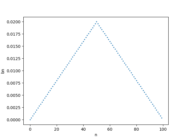
After multiplying samples with those coefficients, we increase amplitude in the middle of our waveform, and decrease amplitude at beginning and at the end. We want filter that have gain of 1 at DC value, so the the sum of all coefficients should be equal to 1. That’s why the highest point in our triangle is 0.02. If we multiply those coefficients by our DC value, and then add all products then (because sum of coefficients is 1) we should get back our DC value
Now let’s take a look how this filter work for 150 Hz. On upper chart there is our 150 Hz signal (black line), but I also put there coefficients of filter (multiplied by 100 to make it visible in that scale). The filter is working as in previous examples, so the coefficients are moving through our signal. On the middle chart, there is drawn signal multiplied by filter coefficients (raw coefficients, not multiplied by 100). On the bottom chart you can see the sum of all points of middle chart which is filter output.
As we can see, the amplitude of 150 Hz signal is about twice lower than in case of just averaging filter. Let’s make another simulation for 450 Hz signal.

This time the amplitude of filter output is much less than in averaging filter (about 10 times). Just to make sure our filter pass the DC voltage I made simulation:
Ok, our filter works well. Anyway in above examples I just wanted to show how digital FIR filter works, and how averaging filter works. Well… the FIR filter (with some nice coefficient values) works better, but averaging require much less calculations.
I hope I didn’t make it more complicated as it is.