
Few days ago I received couple of evalboards from Microchip. One of them is:
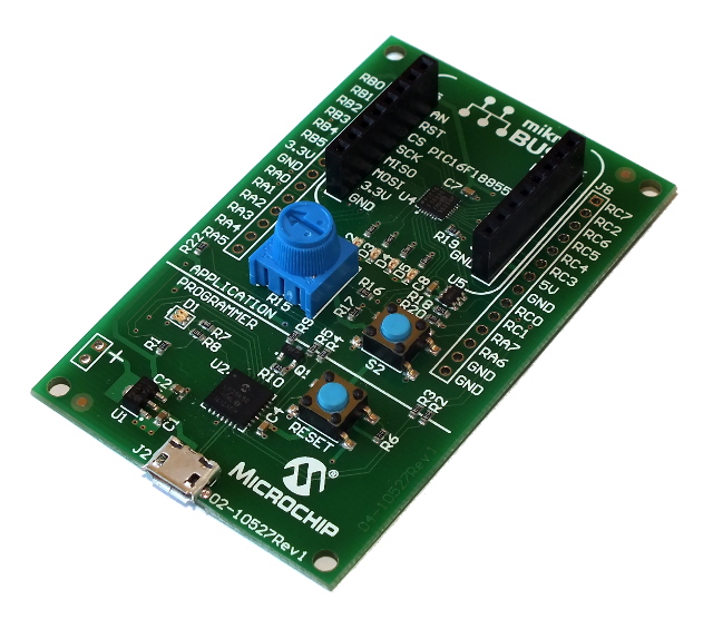
MPLAB® Xpress Evaluation Board (DM164140)
The microcontroller on that board have some nice peripheral called ADC with Computation (ADCC, ADC2). It’s 10 bit ADC that can also make some mathematical operations on samples without using CPU. There are few operations that it can make (Basic, Averaging, Burst averaging, Accumulating, Low pass filter), but I’ll focus on averaging and low pass filter. Averaging is very common technique to reduce noise in DC or low frequency measuring systems. There’s a lot of electronic engineers that using averaging on ADC results at default, before even checking if it’s necessary.
In this test I would like to check those modes. Averaging mode is quite simple to understand after reading the datasheet of microcontroller, but there’s not much information how this low pass filter mode works, so i decided to test and compare it to the averaging mode.
First let’s test ADC with average mode. This mode adds continuously sample values, and then performing right shift on that sum by some numbers of bits. Right shift is actually dividing by:
\(2^{n}\)
n – number of position shifted to right
So in general, we are adding sample values, and then dividing it by 2n. If the number of sample values in the sum are equal to division factor, then we have the average value of those samples.
I wrote small program for the microcontroller that will collect the 128 samples and after that it will send results by UART to computer. Sampling is stopped during sending data by UART (sending time was actually much longer than sampling time, so it wasn’t really good idea to keep sampling during sending data, because new samples would override old samples during transmission).
Sampling period and frequency of our system equals:
\(T_S = 100\, \mu s\)
\(f_S = \frac{1}{T_S} = 10\, kHz\)
TS -sampling period
fS -sampling frequency
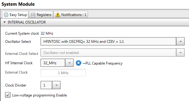
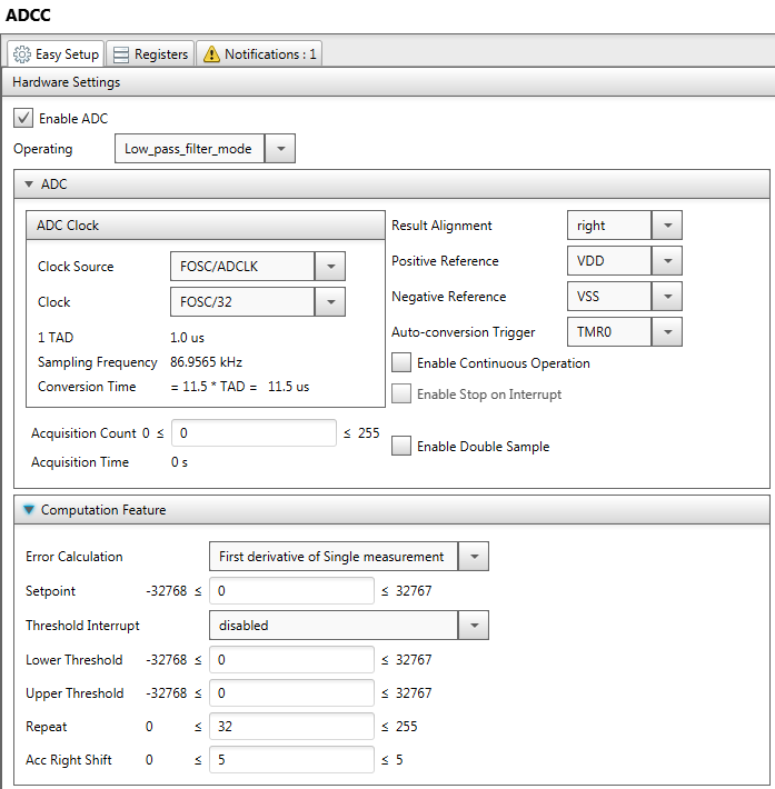
I used MPLAB Code Configurator to create starting point of that program. Configuration is presented below:
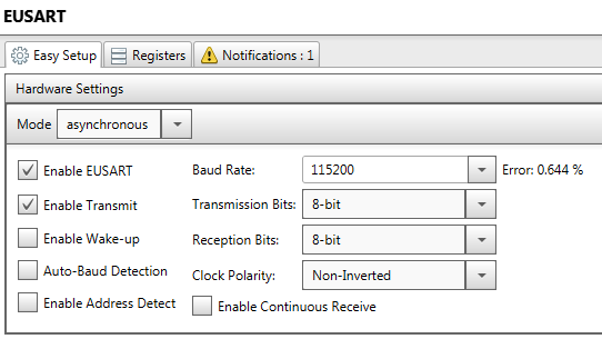
EUSART is used just to sending data.
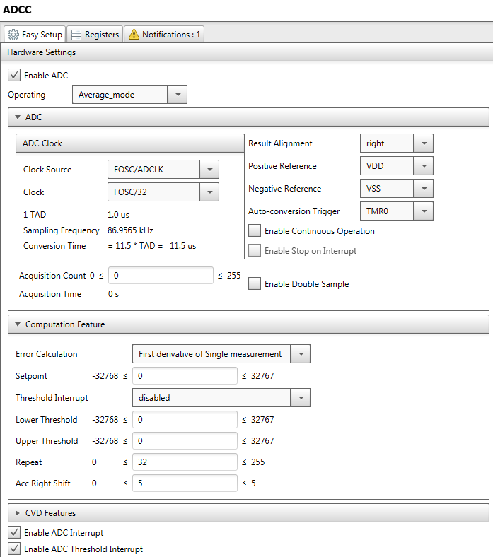
ADC parameters need explanation. It is possible to run ADC continuously by checking the field ‘Enable Continuous Operation’. In that mode, the ADC starts new measurements right after it finish previous one. In that case sampling frequency is dependent to all parameters (ADC clock frequency, clock divider, Acquisition count…). I decided to use TMR0 as Auto-conversion trigger, so I could set the sampling frequency independently. In that case total sampling plus conversion time should be shorter than our TMR0 period (so it could finish previous conversion before it starts next one).
Acc Right Shift is parameter is set to 5, and number of samples to sum is set by ‘Repeat’ parameter to 32, so in that case we’ll get the average value of 32 samples, because:
\(2^5 = 32\)
The sampling period is 100 us, and we have 32 samples for averaging, so we will have average value of 3,2 ms of input signal.
I’m not using ADC Threshold Interrupt, but I enabled it anyway because if I didn’t, I get some compiler error. We’re just using ADC Interrupt.
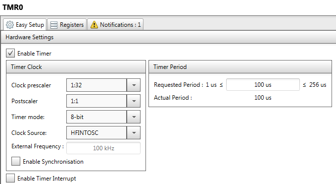
Timer period is set to 100 us to get the sampling frequency of 10 kHz.
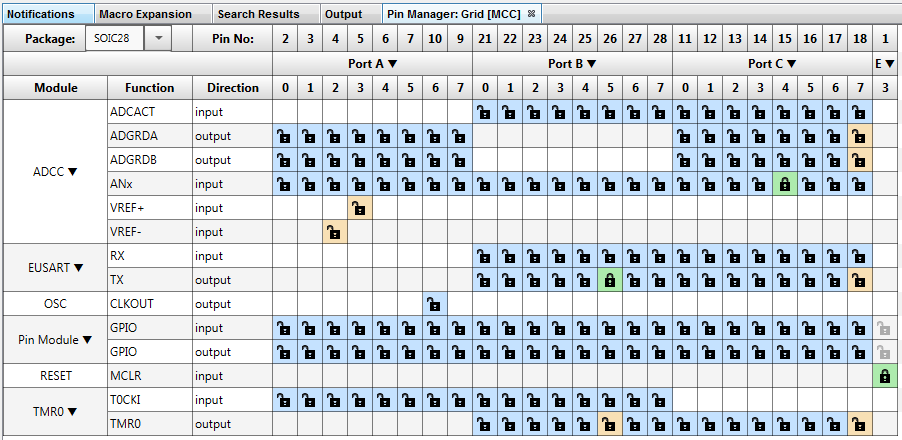
The TX of uart is set to port B pin 5, and input of ADC is on port C pin 4.
I had to modify the main.c file of the project to output the values by EUSART:
#define SAMPLE_ARRAY_SIZE 128

volatile uint16_t results[SAMPLE_ARRAY_SIZE];
volatile uint16_t filtered[SAMPLE_ARRAY_SIZE];
volatile uint16_t accValues[SAMPLE_ARRAY_SIZE];
volatile uint16_t sampleCounter;

void ADCC_IRQ(void)
{
// remember the values of registers used in computation module
    results[sampleCounter] = ((uint16_t)ADRESH << 8)  | ADRESL;
    filtered[sampleCounter] = ((uint16_t)ADFLTRH << 8)  | ADFLTRL;
    accValues[sampleCounter] = ((uint16_t)ADACCH << 8)  | ADACCL;
    sampleCounter++;
// if arrays are full, then stop sampling...
// and send those values by uart
// sending is performed in main function
    if(sampleCounter>=SAMPLE_ARRAY_SIZE)
        TMR0_StopTimer();
}

void sendAllSamples(void)
{
    for(uint16_t i=0;i<SAMPLE_ARRAY_SIZE;i++)
    {
        EUSART_Write(results[i] & 0x00FF);
        EUSART_Write((results[i] & 0xFF00)>> 8);
        for(uint16_t j=0;j<10000;j++);
    }
}

void sendAllFilteredSamples(void)
{
    for(uint16_t i=0;i<SAMPLE_ARRAY_SIZE;i++)
    {
        EUSART_Write(filtered[i] & 0x00FF);
        EUSART_Write((filtered[i] & 0xFF00)>> 8);
        for(uint16_t j=0;j<10000;j++);
    }
}

void sendAllAcc(void)
{
    for(uint16_t i=0;i<SAMPLE_ARRAY_SIZE;i++)
    {
        EUSART_Write(accValues[i] & 0x00FF);
        EUSART_Write((accValues[i] & 0xFF00)>> 8);
        for(uint16_t j=0;j<10000;j++);
    }
}

void main(void)
{
    SYSTEM_Initialize();

    INTERRUPT_GlobalInterruptEnable();
    INTERRUPT_PeripheralInterruptEnable();
    ADCC_SetADIInterruptHandler(ADCC_IRQ);

    sampleCounter = 0;
    ADCC_StartConversion(channel_ANC4);

    while (1)
    {
        if(sampleCounter>=SAMPLE_ARRAY_SIZE)
        {
            sendAllSamples();
// two 0xFF bytes are send after each array to mark the end
            EUSART_Write(0xFF);
            EUSART_Write(0xFF);
            sendAllFilteredSamples();
            EUSART_Write(0xFF);
            EUSART_Write(0xFF);
            sendAllAcc();
            EUSART_Write(0xFF);
            EUSART_Write(0xFF);
            sampleCounter = 0;
            TMR0_StartTimer();
        }
    }
}
ADC is keeping the last value in register ADRESH (higher byte) and ADRESL (lower byte). I will call those registers as ADRES for short. If averaging mode is selected, then with every sample values of ADRES are added to to ADACC registers. In the same time, the ADFLTR is keeping the value of ADACC shifted right by defined value – in our case that value is 5. 5 is maximum numbers of position shifted (in that microcontroller).
In our program, as you can see, we’re collecting values of ADRES, ADFLTR and ADACC at every sampling interrupt (at every new sample) in three arrays:
volatile uint16_t rawSamples[SAMPLE_ARRAY_SIZE];
volatile uint16_t filteredSamples[SAMPLE_ARRAY_SIZE];
volatile uint16_t accumulatedSamples[SAMPLE_ARRAY_SIZE];
After filling those arrays with 128 values, we’re stopping sampling (stopping TMR0) and then we’re sending those arrays by UART. Between every array I put two bytes with values of 0xFF to mark the end of array.
I made also program on PC to get data from UART and write it to text file. UART is connected to PC by FTDI module (it’s not the point of this article, but if you are interested how it’s made feel free to contact me).
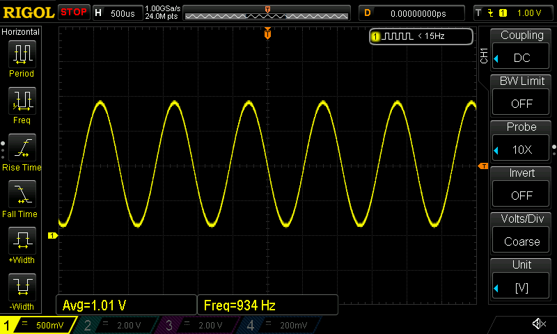
I connected the generator to ADC input and generate signal showed below.
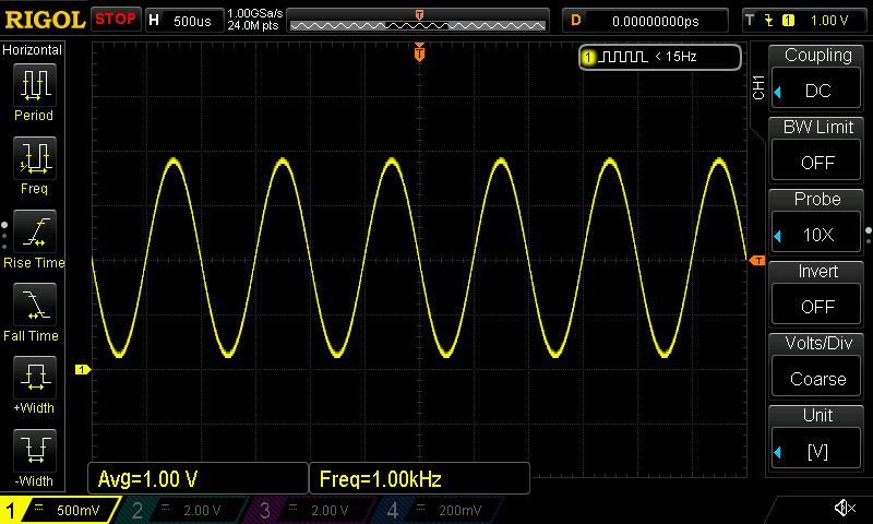
You have to notice that the 0 V (GND level) is not in the middle of scale but two ticks below (the yellow arrow on the left). The average value of this signal (DC component) is 1 V (which is our signal), and AC component is about 1 V, and it’s frequency is 1 kHz (which simulates the noise that we want to filter out).
Now we can turn on our system and get samples of that signal. The 128 samples are showed on the chart below (upper chart). On the same chart I showed also ADFLTR register values.
On the bottom chart, there is accumulated value (ADACC registers).
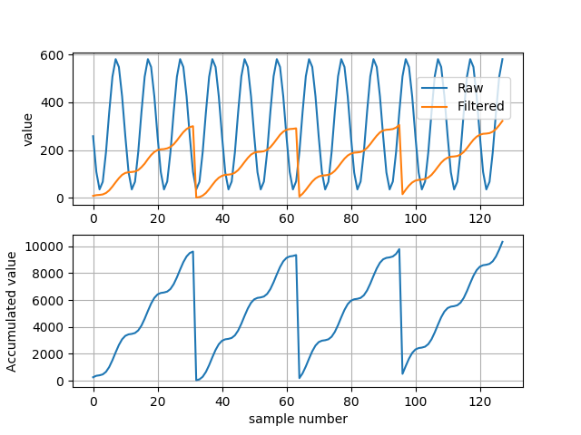
As you can see, the filtered value is available any time, and it’s value is accumulated value divided by 32 (right shifted by 5 positions). Because of that, the average value only have sense at the 32, 64, 96 … sample. Only then in ADACC registers we have sum of 32 samples, so after dividing it by 32 we get average value. We have to ignore all other ADFLTR values. After 32’th sample the value of ADCCH/L register is reset to 0 and accumulation starts again.
If we ignore all filtered values except that at 32, 64, 96 and 128 sample, we get the chart of average values: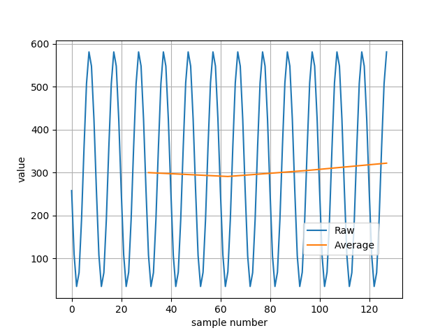
Now there is real average value of our signal. The values on chart is just digital values form ADC, but to check if measuring system works, I calculated voltage from ADC average values.
ADC average values are:
\(AV_1 = 300\)
\(AV_2 = 291\)
\(AV_3 = 305\)
\(AV_4 = 322\)
Voltage levels calculated from reference voltage (which is 3.3 V), and resolution of 10 bit ADC (1023 which is maximum value of 10 bit number) are:
\(V_1 = AV_1 \cdot \frac{3.3\,V}{1023} = 0.968 V\)
\(V_2 = AV_2 \cdot \frac{3.3\,V}{1023} = 0.939 V\)
\(V_3 = AV_3 \cdot \frac{3.3\,V}{1023} = 0.984 V\)
\(V_4 = AV_4 \cdot \frac{3.3\,V}{1023} = 1.039 V\)
The average value of our signal should be exactly 1 V but we have quite large errors. Why? Because we’re averaging signal of 3.2 ms, but one 1kHz sine period takes 1 ms, so we don’t have integer numbers of periods in our averaging range. To check if it we get the exact DC value of our signal, I slightly changed the AC frequency to 937,5 Hz. In 3.2 ms now we should get 3 full sine periods. Again I run the measurements. The signal is showed below:
Sampled and averaged values:
ADC average values are:
\(AV_1 = 309\)
\(AV_2 = 310\)
\(AV_3 = 310\)
\(AV_4 = 310\)
Average voltage levels are:
\(V_1 = AV_1 \cdot \frac{3.3\,V}{1024} = 0.997 V\)
\(V_2 = AV_2 \cdot \frac{3.3\,V}{1024} = 1.0 V\)
\(V_3 = AV_3 \cdot \frac{3.3\,V}{1024} = 1.0 V\)
\(V_4 = AV_4 \cdot \frac{3.3\,V}{1024} = 1.0 V\)
This time I get exactly average value of our signal (actually I was really surprised by that accuracy of measurement).
Now let’s take a look at low pass filter mode.
There is no full information how this filter works in datasheet. Only information I found about mathematics of that filter is showed in table 23-3 (click on it to make it larger):
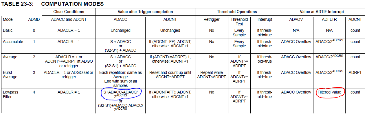 In all modes except the ‘low pass filter’ we have information what is placed in ADFLTR register. Actually that table says what is in that register when ADTIF Interrupt takes place. but for the rest of those modes, it’s also true all the time.
Anyway, that table just says that there is a ‘filtered value’, whatever that means (red mark at the picture). But there is some clue on that table, that helps me to understand how this filter works (equation in the blue mark):
\(ADACC = S + ADACC – \frac{ADACC}{2^{ADCRS}}\)
Well… to explain that, let’s get back to average mode for just a moment. As we saw in previous example, the real average value is in ADFLTR register only after 32 samples. If we want to have average value in every sample, we could use filter called “moving average”. It’s a filter that calculates average value from last defined number of samples. Let’s say that we are calculating average form 5 samples (and actual sample number is 7):
\(AVER_{7} = \frac{x_7 + x_6+x_5+x_4+x_3}{5} \)
xn – value of n’th sample
AVERn – average value form last 5 samples (starting form n to n-4 sample)
As you can see there’s a lot of adding in calculating, and those calculations have to be calculated with every sample. Well… maybe not a lot, but some adding that can be reduced.
Let’s call sum of that sample values (above fraction bar) as:
\(SUM(7..4) = x_7 + x_6+x_5+x_4+x_3\)
Now let’s try to write the same equation for next sample.
\(AVER_{8} = \frac{x_8 + x_7+x_6+x_5+x_4}{5} \)
Again, let’s give a name to that sum:
\(SUM(8..4) = x_8 + x_7+x_6+x_5+x_4\)
Right now, as you can see, we can reduce number of additions in SUM(8..5) by using SUM(7..3} form 4 to 2 (actually 1 sum and 1 subtraction):
\(SUM(8..4) = x_8 +SUM(7..3)-x_3\)
Reduction form 4 to 2 is not much, but if we have sum of 32 numbers, we should get reduction form 32 to 2 so it’s quite large optimization.
Another thing is that we have to keep in memory all 5 sample values, because in next 5 samples we’ll be subtracting that samples from our sum). Is there any other way to avoid keeping that in memory? Let’s say we don’t have all samples in memory, and we just have new sample and previous sum. The best way to approximate that number is make assumption that it is close to average value form our samples, so:
\(x_3 = \frac{SUM(7..3)}{5}\)
Now if we put that value in our SUM(8..4) equation:
\(SUM(8..4) = x_8 +SUM(7..3)-\frac{SUM(7..3)}{5}\)
Have you seen similar equation before? Well it’s almost similar. If we have actually 32 samples we can write that equation as:
\(SUM(8..4) = x_8 +SUM(7..3)-\frac{SUM(7..3)}{2^5} \)
If we call new sample as S, and actual sum as ADACC, and we have 32 samples written as 2^ADCRS (where ADCRS is 5) so we get our equation for ADACC value:
\(ADACC = S + ADACC – \frac{ADACC}{2^{ADCRS}}\)
Now we can guess what that ADFLTR value is. If we want to get DC value at our filter output, and DC value is average value of signal, then we can probably should divide that ADACC register by 2ADCRS:
\(ADFLTR = \frac{ADACC}{2^{ADCRS}}\)
So if it’s true, then in datasheet in ADFLTR column should be that equation in row with low pass filter. The same equation is in all the other columns (except basic mode, but in that mode, there is no calculations).
Ok, now we can check if our theory is right. I modified the program for microcontroller, just by changing mode of ADC to low pass filter:
The rest of configuration is the same. In low pass filter mode, the ‘repeat’ parameter doesn’t matter.
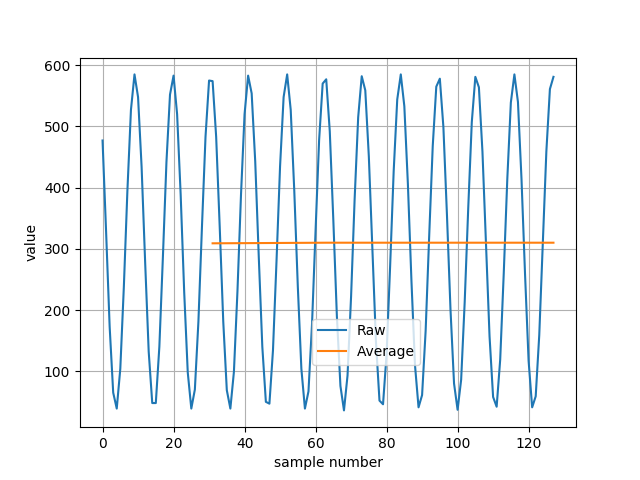
Now I make the same measurements with 1 kHz frequency. Raw samples and filtered samples are showed below.
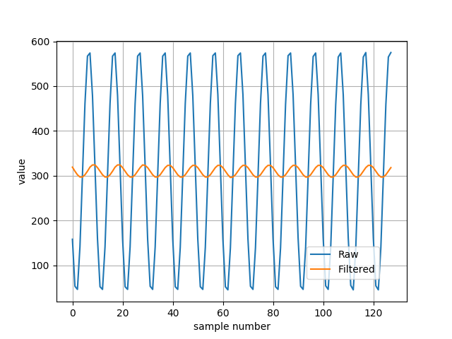 As you can see, the amplitude of AC component is reduced, and DC component of signal is kept. I checked input, output and ADACC values of that filter and I confirmed that it works as I described above. Now we can also check what will happen it we set the frequency to 937,5 Hz like in previous example. Should we get 0 V on AC? Average value from sinus is 0 so probably we should, because equations for that filter is quite close to equation of average value.
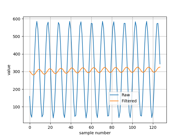 And as you can see… it’s not filtered totally out. Why? Because we made that assumption that we should subtract from our sum the average value instead of real sample value. Because of that we don’t have real moving average filter. That filter is actually called “one pole” IIR filter. IIR stands for Infinite Impulse Response. You can find a lot of information about it in literature or internet. Here I just wanted to show how it’s work in more intuitive way.
Ok, that’s all.
Conclusion.
In both modes (averaging and low pass filter) ADC2 acts as low pass filter. In filter mode we get new output value with every new sample. In averaging mode we get new output value in every 2ADCRS sample.
ADC2 is really useful peripheral, because averaging and low pass filter of measurements is often used in real measurement systems to reduce noise.
There are some more interesting things that can ADC2 can do – like oversampling, accumulating samples etc, but I think that’s enough for this article. I hope you liked it.